Figure fig:type-totals
Total values by Category for a random sample of 18 Type values (out of 31 in all).

In sentiment analysis, one can ignore the pos/neg distinction for only so long ... This section uses words gathered from a large online collection of informal texts to try to build lexical scales. We start by figuring out how best to study word distributions, then look at number of methods (expected categories, logistic regression, and hierarchical logistic regression) for assessing and summarizing those distributions and, in turn, for creating scales from them.
If you haven't already, get set up with the course data and code.
The file ratings-advadj.csv contains data gathered from a wide variety of websites (Amazon.com, OpenTable.com, Goodreads.com, IMDB.com) at which users can write reviews and attach star ratings to those reviews. I think the best way to get a feel for the file is to load it into R and check out its first few lines:
Here's a rundown on the column values:
This concludes our basic tour of the file. Now on to the analyses!
The file ratings.R provides a number of functions for working with the above kind of tabular data. To make these functions available, enter
The structure of the code is strongly reminiscent of the code for the Experience Project data. There are functions for extracting subframes based on various pieces of data, and there are functions for visualizing the relationships between the values. Our focus is again on the Word values, but we will build up to analyses that consider these words in their context, which is here a mix of high-level features and immediate morphosyntactic features.
The function ratingFullFrame is exactly analogous to epFullFrame from ep.R. It extracts subframes based on various supplied parameters. The required arguments are the data.frame and a word or list of words. The other values are optional. Here is a call with all of the default parameter so that you can get a feel for the options:
If ratingmax=5, then the IMDB data are left out. If ratingmax=10, then only the IMDB data are used. Both subsets are substantial, so both can lead to solid results. I often divide the data in this way in order to create prettier pictures.
Arguments that are left with their default values are assumed unspecified, so the data.frame is not restricted based on those values. Where they are specified, the value is limited. Here's an example in which we restrict to situations in which horrid was modified by absolutely:
The Modifier value NONE is special. It groups instances in which Word had no left-adjacent modifiers. Thus, the following gives the purest picture we can get of horrid:
The function ratingCollapsedFrame takes the same required and optional arguments, but it collapses everything down to 10 rows (5 if ratingmax=5), and it has an additional set of optional arguments for adding other values that are useful for modeling (see below).
Recall that the Experience Project data were heavily biased towards the sympathetic categories. A similar issue arises with star-ratings data: essentially all sites on the Internet that collect user-supplied reviews of this form are heavily biased towards positivity. Products that people like are purchased more and hence reviewed more. Products that people dislike are reviewed negatively, which means that fewer people buy them, which reduces the size of the reviewing pool. There is some variation by Type value, but the overall picture is one of relentless positivity.
Thus, if we relied on pure Count values, everything would look positive.
As before, we'll steer around this by using relative frequencies, which we obtain by dividing Count values by corresponding Total values. This can be done directly with ratingCollapsedFrame using the freqs=TRUE flag.
We can also normalize these frequencies as we did before using (Count/Total) / sum(Count/Total), which is an application of Bayes' Rule to the initial probabilities but with the prior over categories flattened out (removed) so that we don't reintroduce the underlying Rating bias. The probs=TRUE flag adds these values to collapsed frames:
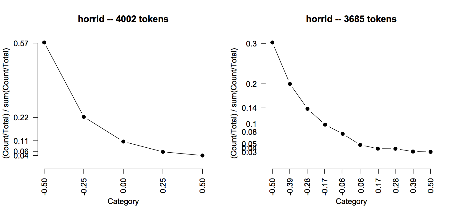
To plot the Freq or Pr values, use ratingPlot, which has the same argument structure as ratingCollapsedFrame, plus optional arguments for setting the limits on the y-axis, the color of the plots, and for depicting model fits (which we will return to below):

The trends are clear, but the plots are a little bumpy due to the way we have combined five-star and ten-star reviews. You can clear this up with the ratingmax parameter if you like:
Exercise ex:words Play around with the ratingPlot, looking systematically at classes of words that you expect to be related, or opposed, when it comes to the polarity scale we are dealing with. This will give you a feel for the data, and also, for better or worse, give you a sense for how small the vocabulary is. It's also a good idea to use the corresponding ratingCollapsedFrame function call to see what the raw data are like.
Exercise ex:shapes It's easy to find words that have strong biases for one end of the scale or the other (pos/neg). Can you find any that are biased towards the middle, or towards the edges together. What are such words like?
Exercise ex:neg Use ratingPlot to study the effects of negation. As a first step, I recommending using modifiers='NONE' to see what the basic distribution of the word is, and then adding modifiers=c("not", "n't", "never"). An example (the results are given in figure fig:good-neg):

Exercise ex:mods Broaden the investigation of negation begun in exercise ex:neg to include other modifiers — perhaps those that you expect to behave differently from negation.
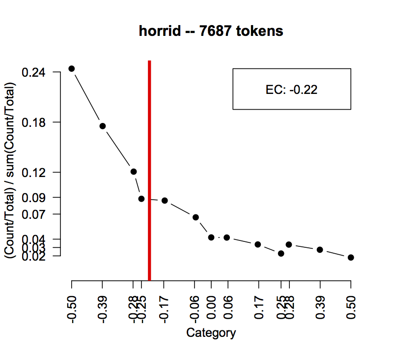
The expected category calculation is just a weighted average of Pr values. It's true to its name in the sense that it provides the best-guess value if someone gave you the word and asked you to select an appropriate Category for it.
The function ExpectedCategory does this automatically:
You can add expected categories to ratingPlot outputs directly:
Exercise ex:er Return to the words you plotted earlier, but now check out their expected categories by adding them with the ec=TRUE flag. Do these values suggest a method for building pos/neg sentiment lexicons?
Expected categories are easy to calculate and quite intuitive, but it is hard to know how confident we can be in them, because they are insensitive to the amount and kind of data that went into them. Suppose the EC for words v and w are both 10, but we have 500 tokens of v and just 10 tokens of w. This suggests that we can have a high degree of confidence in our EC for v, but not for w. However, EC values don't encode this uncertainty, nor is there an obvious way to capture it.
Logistic regression provides a useful way to do the work of ECs but with the added benefits of having a model and associated test statistics and measures of confidence. To start, we can fit a simple model that uses Category values to predict word usage. The intuition here is just the one that we have been working with so far: the star-ratings are correlated with the usage of some words. For a word like horrid, the correlation is negative: usage drops as the ratings get higher. For a word like amazing, the correlation is positive.
With our logistic regression models, we will essentially fit lines through our Freq data points, just as one would with a linear regression involving one predictor. However, the logistic regression model fits these values in log-odds space and uses the inverse logit function (plogis in R) to ensure that all the predicted values lie in [0,1], i.e., that they are all true probability values. Unfortunately, there is not enough time to go into much more detail about the nature of this kind of modeling. Instead, let's simply fit a model and try to build up intuitions about what it does and says:
Here, we use R's glm (generalized linear model) function to predict log-odds values based on Category. The expression cbind(horrid$Count, horrid$Total-bad$Count) is used internally by glm to derive the log-odds distribution. Category is our usual vector of Category values. The family=quasibinomial specification invokes a binomial family of the sort that characterizes logistic regression, but it should give us more conservative p values for our kind of count data than binomial would.
Let's begin by inspecting the coefficients for this fit:
The negative sign on the coefficient for Category squares well with the fact that this is a negative word. If we fit the same model with a positive word, the Category coefficient flips its sign:
The Intercept correlates with overall corpus frequency. We will mostly ignore it.
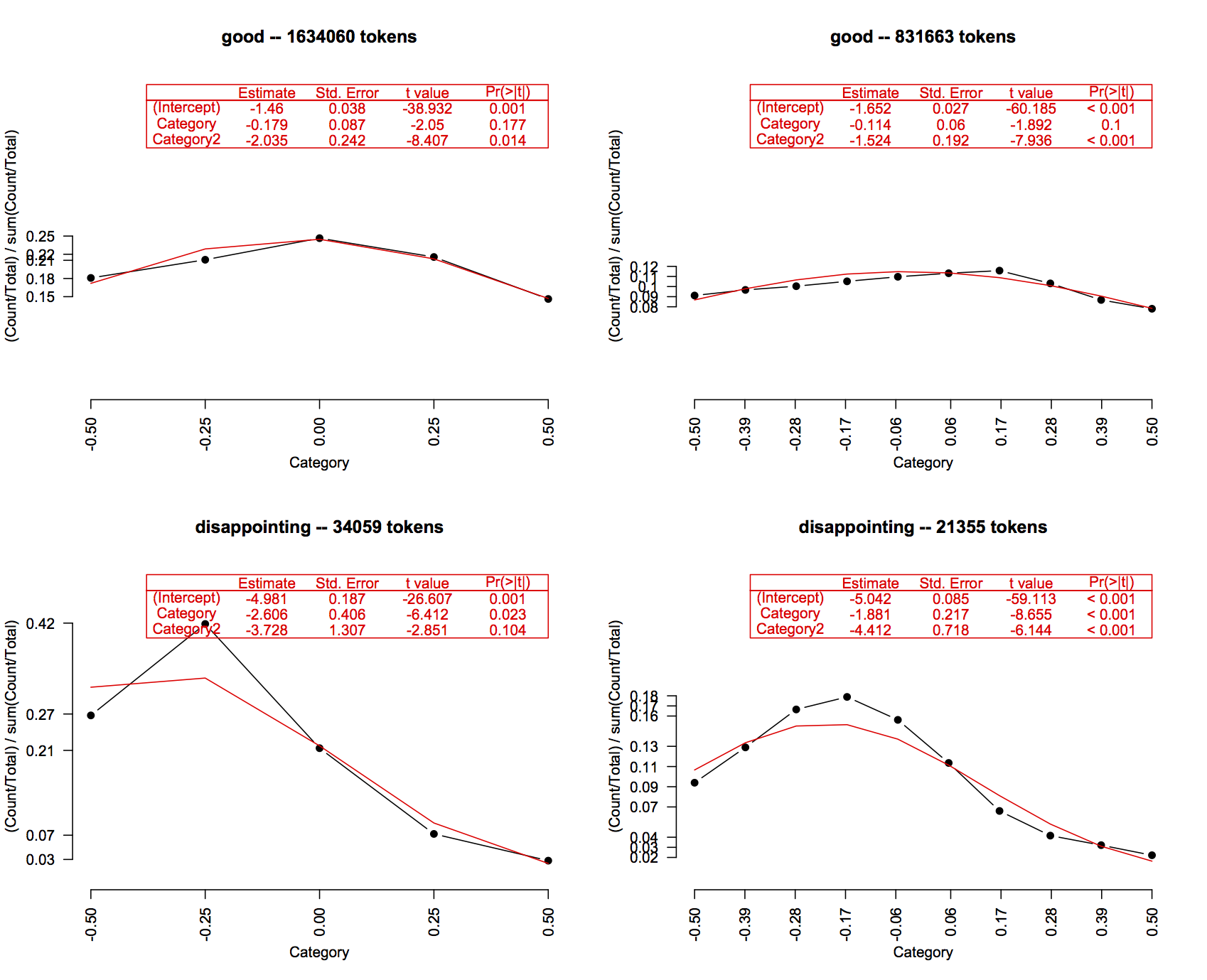
The models are more easily understood when juxtaposed with the empirical estimates on which they are based. ratingPlot makes this easy: it takes an option argument models that can have one or more models as its values. Due to an oddity of the way R stores the values, even single models have to be given inside c() (but no quotes; you're actually passing in the function!). The results of those models will be displayed as part of the empirical plot. You can define your own model functions, but ratings.R also makes some available. GlmWordLinear is the model we've been using so far.

The above models generally look good. In some cases, though, the assumption that frequencies are linearly correlated with the Category is clearly false. For example, good and disappointing are mildly positive and negative, respectively, which gives them an arch-like distribution. This suggests that we would do well to include the squared Category value as a predictor. ratings.R has such a model prespecified: GlmWordQuadratic.
Exercise ex:logit Once again, return to the words you plotted earlier, but now try to determine whether GlmWordLinear or GlmWordQuadratic provide good model fits for them. As you do this, consider which values you might be able to use as sentiment scores.
We can use the EC and logistic regression values to order all the lexical items. First, let's create a separate table containing just the EC value, Category coefficient, and Category p value for each word in the vocabulary. To do this efficiently, I first define an auxiliary function that, given a word's frame, gets these values for us:
The function ddply from the plyr library efficiently handles grouping words (based on Word identity) and sending those subframes to WordAssess for the needed values, then adding them to a data.frame:
It will take your computer a while to generate the values. For safety, save to a file so that you can use it later:
The data.frame ratings.assess has the potential to deliver us a pos/neg sentiment lexicon with continuous values. Here is a flexible function for working with it:
Exercise ex:lexuse Use PosnegLexicon to study the lexicons we can obtain with the above methods. What are their strengths and weaknesses?
Exercise ex:pvals How many of the words in our lexicon have significant Category coefficients? Which words fail to achieve this level? Why?
Exercise ex:corr How do the EC and Category values relate to each other? Are they highly correlated, or not? What kinds of words end up with very different EC and Category values?
Exercise ex:quad The method for generating lexicons defined above does not use the model GlmWordQuadratic, which has an additional predictor for Category. How might we effectively use this model? Should it replace GlmWordLinear, or should we use them both?
Exercise ex:wordcmp The above lexicon-generation method might make statisticians unhappy because, strictly speaking, we can't compare coefficients from different fitted models and draw conclusions about the strength of the effects they capture. However, a simple extension of our basic approach is pretty respectable. The basic strategy is to make pairwise comparisons in the model. To do this, create two collapsed frames pf1 and pf2 using ratingCollapsedFrame, bind them together with pf = rbind(pf1, pf2), and then extend the frame with pf$Stronger = pf$Word == as.character(pf1$Word[1]). Now use Stronger strategically in your model. (If you decide to pursue this question, perhaps write to me — I have some annotated data that can be used for assessment.)
Having generated a lexicon, one naturally wonders how good it is. Luckily, there are existing pos/neg lexicons that we can compare against. Here, I use the very rich MPQA lexicon, which classifies words along two dimensions: positive/neutral/negative and weaksubj/strongsubj. This file is included in today's code distribution:
I've mapped the MPQA string Polarity values into numbers: -1 is negative, 0 is neutral, and 1 is positive. (I'll ignore the Subjectivity values, but I also mapped them to numbers: 1 is weaksubj and 2 is strongsubj.)
The MPQA's vocabulary is very large, and it includes words of different parts of speech. Our lexicon of ratings data contains only adjectives, so I'll restrict the frame to just the adjectival data:
We're now in a position to compare our derived values against the MPQA. The first step is to add an MPQA column to our lexicon frame ratings.assess. I again call on ddply:
The final step is to use our values to make polarity predictions. There are lots of ways we could do this. My initial proposal is to assume that words for which we don't have miniscule p-values are words that are neutral (Category doesn't predict their usage), and then to use the sign of the Category coefficient from there:
The confusion matrix we just created has the gold-standard data going row-wise and our predictions going column-wise. The sum of the diagonals divided by the total is our accuracy:
Accuracy is not the best measure in this case because the gold-standard data are imbalanced, with very few neutral words:
It is better to balance prediction and recall when thinking about how we did:
Clearly, the neutral category is problematic for us. This is because our model predicts this category much more often than it is attested in MPQA. This seems like an inherent drawback to the assessment method: we just have different standards for neutrality at work. (Perhaps we would do better to assess only against the strongsubj cases.) However, the pos/neg confusions should be addressable. Let's look at a random sample of the errors from our worst category in terms of precision:
If one samples around with ratingPlot, it quickly becomes clear that many of the failures are failures of our underlying model: words like sad are too weak to have truly significant linear relationships to the categories. They call for the quadratic model, making it all the more pressing that we figure out a way to bring those values into our lexicon generation method (exercise ex:quad; a hint: both the quadratic and the linear Category coefficients can be used as scores, and they can even be effectively compared, as long as they are normalized somewhat, since the quadratic scores are generally much smaller than the linear ones.)
Exercise ex:assess-ec Add a column ECPrediction to the ratings.assess frame and fill it with EC values, then re-run the assessment. How do the results compare to those obtained with the CategoryCoef values?
Exercise ex:subj The MPQA data.frame also supplies subjectivity values (1 is weaksubj and 2 is strongsubj). Do these value correlate with our sentiment scores?
Exercise ex:op Today's file also contains a CSV file containing the contents of Bing Liu's Opinion Lexicon:. Assess our own lexicon against this.
In the section on Experience Project data, we used first logistic regression and then hierarchical logistic regression to model the relationships between words and contextual variables. I pursue a version of the hierarchical strategy here. The above models are insensitive to all kinds of context, but we've seen already that such variables matter. It's time to bring it in to our models and, in turn, into our lexicons!
ratings.R makes available a few hierarchical models. LmerWordType fits a hierarchical model that uses Category as the sole fixed-effects predictor and Type as its sole hierarchical predictor. This model delivers a fixed effects estimate for Category (a kind of weighted average over the different subclasses given by Type), and it also provides such estimates for the intercept and Category values for each value of Type. Thus, we have one pooled model (fixed effects) and 1 model for each of the 31 different Type values:
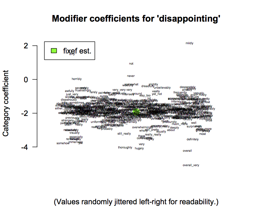
The function ratingPlotHierarchicalCoefficients plots the fixed and hierarchical coefficients. The result is a ranking, top to bottom, but with the labels jittered randomly left to right so that nearby values don't sit ontop of each other. The fixed-effect estimate is given as a big green dot:

The model LmerWordModifier uses the same technique, but with Modifier as the hierarchical effect. The results provide a glimpse of the multifaceted ways in which adverbs modulate the meanings of the words they modify.
Exercise ex:modshapes The ModifierType values are shapes that correspond intuitively to the picture we get when regressing the frequency of Modifier on Category or Category2. These provide rough semantic classifications, and the resulting models are more constrained than those obtained directly from the modifiers. ratings.R contains a model LmerWordModifierType for exploring these values with respect to specific words. Use ratingPlotHierarchicalCoefficients to get a feel for what the shapes are like and how they might be used in semantic/sentiment analysis.
Exercise ex:neg-estimates Use the above modeling techniques (any of them) to study the effects of negation. Are there generalizations we can make about how negation affects the sentiment scores we can derive from these data?
Exercise ex:larger The vocabulary of ratings-advadj.csv might start to feel confining after a little while. The file imdb-unigrams.csv in the code distribution for my SALT 20 paper is compatible with the above functions. It doesn't have the contextual features, but it has a truly massive vocabulary: potts-salt20-data-and-code.zip.
Exercise ex:assess-lmer As a first step towards building a context-aware lexicon, adapt the scale generation method of section 7 above to the hierarchical setting by using the fixef coefficients in place of the GLM ones, using one of the lmer models discussed above. Then assess the resulting lexicon against the MPQA as in section 8.
Home
 This work is licensed under a Creative Commons Attribution-NonCommercial-ShareAlike 3.0 Unported License.